Systematic match inspection

Although the DNASAND and the ZEBRA algorithm do not specify the overall type of global relationship of two sequences (total correspondence, containment or overlapping, see Huang (1994)), any type of relationship is recognised. As result of this first scan, a hash storing technique is used to represent sparse matrices containing information on potential overlaps of all the fragments and their orientation (forward-forward or forward-complement) is generated. Figure 23 shows a schematic drawing on how these data structures are interpreted internally.

Figure 23: The ``matrices'' generated after the first fast scan of every read against every other in search for potential overlaps. Unlike this small example with 6 reads might suggest, the matrices in real world projects - with a large number of reads - are normally sparsely occupied. Therefore, using hash storing techniques is more appropriate as otherwise memory consumption would explode for larger number of reads.

In the next fundamental step, these potential overlaps found during the scanning phase must be examined more thoroughly. Several algorithms have bee devised for alignments of multiple sequences: Allison (1993) devised a divide-and-conquer technique for aligning three strings, Stoye (1998) used a similar technique for 6 to 12 strings. But these multiple alignment algorithms are still too slow (see Gotoh (1993) for a good explanation) to be used in an assembly match inspection phase, even when parallelised multiple alignment algorithms run on multiple processors like Kleinjung et al. (2002) presented.

In the end, the strategy devised for the mira assembler works by examining potential matches two at a time with a modified Smith-Waterman algorithm for local alignment of overlaps. Similar strategies were extensively studied by Barton (1993) and have found their way into other current assemblers like, e.g., PGA (Paracel (2002b)).

Improving Smith-Waterman alignment by banding

Observe that two sequences that align well will generate a path through a Smith-Waterman alignment matrix that will almost run diagonally from the entry point to the exit point. Only indels will cause a horizontal or vertical shift of the alignment graph. Assuming that one knew the approximate whereabouts of either the entry or the exit point and that the alignment has 'acceptable' quality, i.e. not too many indels that are spread unilaterally in one of the sequences. It is then a valid assumption that it should be feasible to reconstruct the alignment by calculating only the narrow corridor (a band) through the matrix where the alignment graph is expected to run through, as is shown in figure 24.

A bonus information not to be underestimated is the fact that both DNASAND and ZEBRA not only provide the information whether two sequences are similar enough to try a sequence alignment, but they also provide the approximate offset for the sequence alignment. This information is valuable because it locates the approximate entry points of such an alignment in the alignment matrix and therefore allows to reduce the computational complexity - and with it the time needed - for a SW alignment with two sequences drastically.

Figure 24: Smith-Waterman banding. n₁ and n₂ are the length of the sequences. Instead of computing the whole matrix (n₁*n₂ cells), only a small band within the approximated area of the overlap must be computed: o is the approximated offset from sequence 1 to sequence 2 in the alignment, m the approximated length of the overlap and k the band width to be calculated. s is the predicted starting point for the recursive path drawing algorithm and e the predicted exit area.

Let n₁ and n₂ be the length of the sequences, m the approximate length of the overlap and k a safety margin of indels that might arise in the alignment of the overlap. It is clear that

m $$\leq$$ min(n₁, n₂)

is always true for every possible configuration of m, n₁ and n₂. Furthermore one can assign k to be

k = $${\frac{{1}}{{10}}}$$*m        where typically        30 $$\leq$$ k $$\leq$$ 70

The higher k, the more tolerant the algorithm will be regarding slightly false approximations of alignment path entry-points or the more non-compensated indels can occur in one of the sequences. Using the values mentioned above ensures a sufficiently wide and adaptable security margin for the length of sequences that have to be aligned in a shotgun assembly while keeping k linear within bounds.

While the normal Smith-Waterman alignment will need O(n₁*n₂) time to compute the alignment matrix, the banded version will need only

O(k*m) $$\lessapprox$$ O($${\frac{{1}}{{10}}}$$m²)

to compute the band through the matrix where the alignment is supposed to be. For n₁, n₂ being typically between 300 and 1200 and normally

m $$\ll$$ n₁*n₂

so O(k*m) can be seen to have mostly a less than linear complexity compared to the square complexity of O(n₁*n₂).

Note that although methods for linear-space alignment methods have been devised²³, these have not been implemented for the time being as typical shotgun fragment lengths are small enough to allow quadratic space algorithms.

Figure 25: Smith-Waterman band prediction. According to the offset prediction from DNASAND and ZEBRA-BLOCKING (examples o₁, o₂ and o₃ in the figure), different bands can be computed, all differing in length. These examples show particularly well how the O(n²) Smith-Waterman calculation of a matrix can be effectively scaled down to less than O(n).

The changes needed to adapt the SW algorithm are minimal. A small logical overhead is needed to segment the band and the matrix to facilitate computation. Additionally - and assuming the alignment matrix is calculated row by row - the left and right edge of each row must calculated with a slightly adapted algorithm to take care that the recursive alignment algorithm afterwards will not run out of the band.

Cells outside the calculated band are assigned to have a very high value, e.g. the INTMAX value, which is defined to be the highest integer value that can be represented within a given integer datatype. In practice, to avoid the O(n²) complexity of filing the whole matrix, only the matrix cells adjacent to the calculated band are initialised. This constitutes a 'fence' that the recursive path alignment algorithm will not be able to transgress later on and make sure that all alignments found later will stay within the calculated band.

Figure 26: Smith-Waterman (SW) band calculation predecessor rules. The figure shows a section of a larger SW matrix. The grey cells represent the border of the band within the matrix, arrows show the predecessor cells needed to compute a cell. Most cells in a band will be of type (a), i.e., cells with normal predecessor rules like in a normal SW matrix. Cells on the border of the band (b) and (c) need special handling as they only have two (different) predecessor cells instead of three.

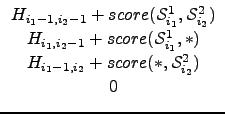
The calculation of cells that are not on the edges (the 'a' cell in figure 26) is performed like in a normal SW algorithm:

H_{i1, i2} = max$$\left\{\vphantom{ \begin{array}{c} H_{i_{1}-1, i_{2}-1} + score(... ...ensuremath{*}, \ensuremath{\mathcal{S}_{i_2}^{2}})\\ 0 \end{array} }\right.$$$$\begin{array}{c} H_{i_{1}-1, i_{2}-1} + score(\ensuremath{\mathc... ...+ score(\ensuremath{*}, \ensuremath{\mathcal{S}_{i_2}^{2}})\\ 0 \end{array}$$$$\left.\vphantom{ \begin{array}{c} H_{i_{1}-1, i_{2}-1} + score(\... ...nsuremath{*}, \ensuremath{\mathcal{S}_{i_2}^{2}})\\ 0 \end{array} }\right\}$$

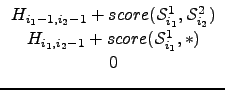
while each cell on the left edge in a row (the 'b' cell in figure 26) must not consider the fence value to its left and consequently is calculated using

H_{i1, i2} = max$$\left\{\vphantom{ \begin{array}{c} H_{i_{1}-1, i_{2}-1} + score(... ...ensuremath{*}, \ensuremath{\mathcal{S}_{i_2}^{2}})\\ 0 \end{array} }\right.$$$$\begin{array}{c} H_{i_{1}-1, i_{2}-1} + score(\ensuremath{\mathc... ...+ score(\ensuremath{*}, \ensuremath{\mathcal{S}_{i_2}^{2}})\\ 0 \end{array}$$$$\left.\vphantom{ \begin{array}{c} H_{i_{1}-1, i_{2}-1} + score(\... ...nsuremath{*}, \ensuremath{\mathcal{S}_{i_2}^{2}})\\ 0 \end{array} }\right\}$$

Similarly, each cell on the right edge in a row (the 'c' cell in figure 26) must not consider the fence value to its top, so that the calculation is done using

H_{i1, i2} = max$$\left\{\vphantom{ \begin{array}{c} H_{i_{1}-1, i_{2}-1} + score(... ...ensuremath{\mathcal{S}_{i_1}^{1}}, \ensuremath{*})\\ 0 \end{array} }\right.$$$$\begin{array}{c} H_{i_{1}-1, i_{2}-1} + score(\ensuremath{\mathc... ...+ score(\ensuremath{\mathcal{S}_{i_1}^{1}}, \ensuremath{*})\\ 0 \end{array}$$$$\left.\vphantom{ \begin{array}{c} H_{i_{1}-1, i_{2}-1} + score(\... ...nsuremath{\mathcal{S}_{i_1}^{1}}, \ensuremath{*})\\ 0 \end{array} }\right\}$$

Parametrising Smith-Waterman alignment

Several scoring schemes for SW alignments have been devised within the last two decades, ranging from the simple original one (Smith et al. (1981)) to methods accounting for gap lengths using affine gap calculation and even alignments of sequences against trace signals. Most publications that appeared analyse and discuss the complexity of dynamic programming and scoring functions. Even very formal but systematic and generally applicable methods to build early prototypes for these algorithms were presented (see also Giegerich (2000)). Althaus et al. (2002) proposed a multiple sequence alignment (MSA) with arbitrary gap costs which computes an optimal solution using polyhedral combinatorics, but having only two sequences at a time to score.

Arslan et al. (2001) presented a method that used iterated Smith-Waterman computations with fractional programming with a run time of O(n²log(n)) - which is already higher than the O(n²) of standard Smith-Waterman - to normalise the score of sequence alignments. Their experimental results suggested that the number of required iterations were small, but they could not establish a satisfactory theoretical lower- / average- / upper-bound for the growth in the number of iterations needed.

Good alignments base on an appropriately chosen scoring scheme given to an optimisation model. A slightly improved original Smith-Waterman scoring scheme has been opted for simplicity, speed and sufficient sensitivity and specificity of a first alignment approximation. The Smith-Waterman alignment algorithm uses the weight matrix W given in table 2 to calculate an alignment score.

[Used SW scoring weight matrix]Extend version of the matrix shown in table 1. Here, comparisons of $\mathcal {A}$^b with endgaps ($\nabla$) or with ``N'' are score neutral.

	A	C	G	T	N	*	$\nabla$
A	1	-1	-1	-1	0	-2	0
C	-1	1	-1	-1	0	-2	0
G	-1	-1	1	-1	0	-2	0
T	-1	-1	-1	1	0	-2	0
N	0	0	0	0	0	-2	0
*	-2	-2	-2	-2	-2	0	0
$\nabla$	0	0	0	0	0	0	0

As can be seen by the values of W, this scoring scheme reflects ideally the requirements that alignments of shotgun sequences with some degree of errors contained: one can assume a 'mismatch' of a base against a 'N' (symbol for aNy base) to have no penalty as in many case the base caller rightfully set 'N' for a real, existing base (and not an erroneous extra one) that could not be resolved further. But to show that this still constitutes a minor reason for being careful, a 'N' gets a neutral score instead of a match.

The scoring algorithm can be improved further by taking into account that - regarding the fact that todays base callers have a low error rate - the block-indel model (see Giegerich and Wheeler (1996)) does not apply to the alignment of shotgun sequencing data: long stretches of mismatches or gaps in the alignment are less probable than small, punctual errors. In fact, more than two gap symbols following each other in an alignment of shotgun sequences is a distinct signal that either the sequences should probably not be assembled together or that something went wrong in the laboratory or during signal processing (base calling). For this reason, a configurable penalty function has been added that scales down the score calculated through the scoring matrix W in relationship to the number and length of gaps within an alignment. The penalties used are shown in table 3. This is a post-processing normalisation algorithm which is not dissimilar to the methods proposed by Pearson (1995) and Shpaer et al. (1996).

[Default gap length penalty scores]Default penalty scores inflicted to the score calculated with a weight matrix. Each gap of a given length reduces the original score by a specified penalty.

gap length in bases	penalty in %
1	0
2	5
3	10
4	20
5	40
6	80
7+	100

In addition, a second score - the expected score - is calculated using the score matrix represented in table 4.

Scoring weight matrix for the expected score

	A	C	G	T	N	*	$\nabla$
A	1	1	1	1	0	1	0
C	1	1	1	1	0	1	0
G	1	1	1	1	0	1	0
T	1	1	1	1	0	1	0
N	0	0	0	0	0	1	0
*	1	1	1	1	1	0	0
$\nabla$	0	0	0	0	0	0	0

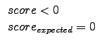
It can be deduced by the matrix values that this second score represents the score expected if the alignment was perfect, i.e., without errors. Consequently

score $$\leq$$ score_expected

is always fulfilled. Note that it is not possible to take the length of the overlap as expected score, because 'N' bases are treated as neutral in score calculation. They therefore cannot get a better score in the calculation of the expected score as this would mean there is an error although it is still assumed that an 'N' is a correctly found base.

Attributing an alignment overlap

It is now trivial to make a ``rough guess'' of the alignment quality of the overlap by calculating the score ratio.

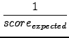
R_s = $${\frac{{1}}{{score_{expected}}}}$$*score        with R_s = 0 for $$\left\{\vphantom{ \begin{array}{l} score < 0\\ score_{expected} = 0\\ \end{array}}\right.$$$$\begin{array}{l} score < 0\\ score_{expected} = 0\\ \end{array}$$

and therefore

0 $$\leq$$ R_s $$\leq$$ 1

A score ratio of 0 shows that the two sequences do not form a valid alignment while a ratio of 1 means a perfect alignment without gaps or base mismatches.²⁴

A problem left open up to now is the question on how to subsume the different quality criteria i) length of the overlap and ii) score ratio into one pregnant figure (the overlap weight) so that overlaps can be ranked easily and comprehensibly.

The simplest method would be to multiply both values to get a weighted length of the overlap. Let len_o be the length of the overlap, so the desired weight w_o of this overlap could be computed by

w_o = len_o*R_s

But this approach attributes far too much weight to the length than it does to the score ratio, which is - after all - the predominant measure for the quality. For example, an overlap of length 650 bases with a score ration of only 0.65 (65% similarity) would get a higher weight (422) than an undeniably better overlap of length 400 bases and a score ratio of 0.9 (90% similarity, weight: 360). This problem can be easily circumvented by squaring the score ratio, giving it more importance in the calculation:

w_o = len_o*$$\left(\vphantom{R_{s}}\right.$$R_s$$\left.\vphantom{R_{s}}\right)^{2}_{}$$

The first overlap would then get a weight of 274 and the second 324, which is exactly the desired outcome.

Every candidate alignment overlap pair whose score ratio is within a configurable threshold (normally upward of 70% to 80%) and where the length of the overlap is not too small is accepted as 'true' overlap, candidate pairs not matching these criteria - often due to spurious hits in the scanning phase - are identified and rejected from further assembly (see figures 27 and 28).

Figure 27: A modified Smith-Waterman algorithm for local alignment is used to confirm or reject potential overlaps found in the fast scanning phase. Accepted overlaps get a weight assigned depending on the length of the overlap and alignment quality.

Figure 28: Although having a good partial score, the overall score ratio of this alignment is too low to be accepted. This read pair is eliminated from the list of possible overlaps.

Building a graph

The overlap alignment - along with complementary data (like orientation of the aligned reads, overlap region, score, score ratio etc.) - is called an aligned dual sequences (ADS). Every ADS that passed the Smith-Waterman test is kept in memory to facilitate and speed up the next phases. Good alternatives are also stored to enable alternative alignments to be found later on in the assembly.

All the ADS form one or several weighted graphs which represent the totality of all the assembly layout possibilities of a given set of shotgun sequencing data (see figure 29). The nodes of the graph are represented by the reads. An edge between two nodes indicates that these two reads are at least partially overlapping and can be aligned. Each graph sketches the alignment possibilities of reads for at least one contig. Hence, the number of non-connected graphs is equivalent to the minimum number of contigs the assembler will be able to build.

Figure 29: An overlap graph generated from the aligned overlaps that passed the Smith-Waterman test. The thickness of the edges represents the weight of an overlap. Although the (1,6) overlap is marked for demonstration purposes in this figure, rejected overlaps (due to spurious hits in the scanning phase, see figure 23) are not present in the graph.

The edges themselves are attributed with the score weights computed for the overlaps and stored in the ADS.