Definitions and methods

A genome physically and chemically consists of tightly coiled strands of deoxyribonucleic acids (DNA) which is normally organised in a twisted double helix. The actual information contained in DNA is encoded by four different nitrogenous bases: Adenine (A), Cytosine (C), Guanine (G) and Thymine (T).

Definition 1 (Alphabet)   An Alphabet $\mathcal {A}$includes the characters needed for textual representation of DNA.

In a DNA helix, each base will always pair with its complementary base.

Definition 2 (Complement base)   The complement base of Adenine is Thymine, the complement base of Cytosine is Guanine. If b defines a base, $\overline{{b}}$ represents its complement.

The bases are arranged along a sugar-phosphate backbone. The information needed to create any organism is specified by the sequence of bases - and the molecular structure defined by it - within the DNA. Refer to Bruce et al. (1994) for more information on working mechanisms of nucleic acids in general.

Definition 3 (Sequence)   A sequence $\mathcal {S}$is an ordered succession of characters from $\mathcal {A}$.

As will be explained later on, extracting DNA sequence information from cells is a tedious process involving many different steps. Each of these steps is prone to errors. Due to these errors, uncertainties remain once a sequence has been determined.

Definition 4 ( $\mathcal {A}$^x)   The alphabet $\mathcal {A}$exists through different representations $\mathcal {A}$^x to meet the needs of real world data sets used in assembly processes.

$\mathcal {A}$^b contains only those characters that are needed to represent the discrete DNA sequence as it is found in cells. $\mathcal {A}$^b = {A, C, G, T}

$\mathcal {A}$ⁿ extends $\mathcal {A}$^b with the character N (aNy) which shall stand for bases that could not be determined more specifically in the analysis process. $\mathcal {A}$ⁿ= {A, C, G, T, N}

$\mathcal {A}$^g extends $\mathcal {A}$ⁿ with the gap character ``*'' which implies missing bases within a sequence $\mathcal {S}$. ``*'' is also sometimes denoted as padding character. $\mathcal {A}$^g= {A, C, G, T, N, *}

Please note that $\ensuremath{\mathcal{A}^{b}}\subset\ensuremath{\mathcal{A}^{n}}\subset\ensuremath{\mathcal{A}^{g}}$

Beside these alphabets, a lot of other different alphabets have been created to meet the needs of specific employments, from which the IUPAC (International Union of Pure and Applied Chemistry) code is the most notable. The IUPAC code describes any uncertainty with one character.⁵

Definition 5 (Length of a sequence $\mathcal {S}$)   The length of a sequence is the number of characters $\in$ $\mathcal {A}$of a sequence $\mathcal {S}$. The length is denoted by | |. Please note that $0 \le \ensuremath{\mid \ensuremath{\mathcal{S}}\, \mid} < \infty$

With the help of the definition for the length of a sequence, the raw definition of a sequence can be refined.

Definition 6 (Sequence $\mathcal {S}$^x)   A sequence $\mathcal {S}$^x is an ordered succession of characters from $\mathcal {A}$^x.

$$\ensuremath{\mathcal{S}_{}^{x}} = \left( \begin{array}{ccc} ... ...} \quad\mbox{and}\quad s^x_i \in \ensuremath{\mathcal{A}^{x}}$$

Definition 7 (Reverse complement)   The reverse complement $\overline{{\mathcal{S}}}$ of a sequence $\mathcal {S}$is constructed by writing the sequence $\mathcal {S}$backwards and replacing the bases by their complement. The special characters ``*'' and īNī do not get replaced.

$$\ensuremath{\overline{\mathcal{S}_{}^{x}}} = \left( \begin{a... ...{s^x_{n}}, & \ldots, & \overline{s^x_{1}} \end{array} \right)$$

The length of DNA sequence of organisms present on earth ranges from a few hundred kilobases up to several gigabases. For example, the bacterium Helicobacter pylori 26695 (GenBank accession number AE000511) has 1,667,867 bases (1.7 megabases) in its form as completed on September 7, 2001. In contrast, the human genome consists of approximately 3 gigabases.

But the gel or capillary electrophoresis technologies used to analyse DNA sequences can determine only about a maximum of 1,000 to 1,500 consequent bases, the high quality stretch with low error probabilities for the called bases often being around the first 400 to 500 bases. The problem to be solved is to find a method that allows the sequencing of long genomes, with the limiting factor that no subsequence to be analysed may be longer than 1 to 1.5kb.

Definition 8 (Shotgun method)   The shotgun method consist of cloning and analysing short overlapping DNA fragments randomly generated from a genome (see also DOE (1992)) and subsequently reassembling back in silico the experimentally gained sequences through computational methods.

Figure 1: Simplified shotgun fragmentation sequence analysis. A DNA is cloned and fragmented. Fragments too long for electrophoresis are filtered, the remaining fragments are sequenced. The original DNA sequence must be reconstructed through computational methods by analysing overlapping regions between fragments. In some cases, no fragment covers certain parts of the original DNA sequence, which results in a gap.

A simplified overview on the principles of the shotgun methods is given in figure 1. The DNA to be sequenced is first purified and amplified through cloning and then randomly fragmented into small parts, for example through sonication or the use of restriction enzymes. The fragments, also called inserts, are then sorted by size into so-called clone libraries of different sizes. For example, a genome sequencing project might use four clone libraries, where the fragments of the first library are approximately 2 kilobases in size, the second has 5 kilobases, the third 10 kilobases and the last 50 kilobases.

With the sensitivity levels of current sequencing technology, any type of nucleic acid sequence that is to be sequenced must first be amplified prior to its determination. This is done by inserting the fragment (insert) into a so-called cloning or sequencing vector and then inserting the resulting construct (a plasmid) into host cells - e.g. a bacterium like E. coli - for amplification as is shown in figure 2.

Figure 2: Amplification of DNA through vectors. Small DNA fragments can be easily amplified by attaching it to a vector sequence. The vector/payload construct is called plasmid and is inserted into a bacterial host, the vector gives it the ability to be replicated together with its host.

Definition 9 (Sequencing or cloning vectors)   Vectors are small fragments of DNA - often derived from viruses or bacterial phages - that have the intrinsic capability to replicate themselves and the sequence that is eventually attached to them. The payload sequence is also called ``insert'', its length ``insert size''.

The construct plasmid is then introduced into a host cell , where it replicates together with the cell.

Once each vector/payload construct is amplified enough, a labelled polymerase replication process is started in the known sequencing vector part in forward and reverse direction as shown in figure 3. When using the chain termination dideoxy method published by Sanger et al. (1977), the replicates are terminated by dideoxynucleotides labelled with a fluorescent dye, a different dye for each terminating base. Each replicate will terminate at a different position of the fragment as the dideoxynucleotide prevents the polymerase from continuing the synthesis.

Figure 3: Simplified illustration of location of forward and reverse reads on plasmids. Amplified plasmids are extracted from the host cells and linearised. Then a chain-termination dideoxy polymerase reaction produces fluorescent labelled replicates of different sizes in forward and reverse direction that can be analysed by electrophoresis.

The combined replicates are then separated according to length in a gel or capillary electrophoresis process. The identity of a terminating base from a particular replicate can be detected by a two- or four-channel laser scanner as peak a in the fluorescence signal in the base specific channel. As short replicates will travel faster through the electrophoresis medium, the order of the replicates that pass the scanning mechanism also determines the order of the bases in each insert and thus the order of bases in the DNA fragment sequence.

Definition 10 (Trace)   The DNA signal gained through electrophoresis is called a trace. Each base (A, C, G and T) has its own signal trace, but they are frequently shown superposed as shown in figure 4.

Figure 4: Example for trace data with the four gel lanes superposed.

Although trace signals are the most accurate representation of the sequences that have been analysed (see figure 4), they tend to be impractical as a basis for upcoming computational steps. Further on, genomes are a discrete ordered sequence of the four nucleotide bases. The trace signals must therefore be analysed to extract the original sequence.

Definition 11 (Base-calling)   Base-calling is the process by which a sequence $\mathcal {S}$^b represented by a signal trace T is deduced from the signals. Usually, the alphabet $\mathcal {A}$ⁿ has to be used to generate a sequence $\mathcal {S}$ⁿ as the trace data is not always unequivocal.

Please refer to section 2.2 for a more in-depth discussion on the origin and the problems caused by wrong base calls.

Definition 12 (Read)   A read is composed by the sequence $\mathcal {S}$ⁿ and the trace data from which it has been inferred. Additionally, data gained by preliminary analysis of the sequence - like sequencing vector pollution - or data from other sources - like chemistry and gel used - can augment the information present.

The read sequences extracted from the forward polymerase replication (called forward reads) and the reverse polymerase replication (called reverse or complement reads) are all contained in the original DNA sequence of interest and are supposed to cover it completely in an overlapping way multiple times. But this is a working hypothesis only, based on stochastic assumptions. Although the fragments are assumed to be distributed uniformly along the DNA sequence (Idury and Waterman (1995)), chemical properties of biological sequences occasionally introduce a bias. In real-world projects, the reads will probably leave some gaps in the DNA sequence to be analysed, sometimes due to chemical properties of the sequence at this place (like coiling of DNA), sometimes just due to 'bad luck'. To reconstruct the original DNA sequence by computational means, the relative order and orientation ⁶ of the fragments must be determined. This inference is done using alignment algorithms.

Definition 13 (Alignment)   An alignment is a 2-dimensional matrix formed by k sequences $\mathcal {S}$^x.

$$\bf L \left(\vphantom{ \begin{array}{c} \ensuremath{\mathcal{S}_{1}^{x}} \\ \vdots\\ \ensuremath{\mathcal{S}_{k}^{x}} \\ \end{array}}\right. \begin{array}{c} \ensuremath{\mathcal{S}_{1}^{x}} \\ \vdots\\ \ensuremath{\mathcal{S}_{k}^{x}} \\ \end{array} \left.\vphantom{ \begin{array}{c} \ensuremath{\mathcal{S}_{1}^{x}} \\ \vdots\\ \ensuremath{\mathcal{S}_{k}^{x}} \\ \end{array}}\right)$$ = (1)

which can also be written as

$$\bf L \left(\vphantom{ \begin{array}{ccc} s_{11} & \ldots & s_{1n}\\ \vdots & \ddots & \vdots\\ s_{k1} & \ldots & s_{kn}\\ \end{array}}\right. \begin{array}{ccc} s_{11} & \ldots & s_{1n}\\ \vdots & \ddots & \vdots\\ s_{k1} & \ldots & s_{kn}\\ \end{array} \left.\vphantom{ \begin{array}{ccc} s_{11} & \ldots & s_{1n}\\ \vdots & \ddots & \vdots\\ s_{k1} & \ldots & s_{kn}\\ \end{array}}\right)$$ = (2)

It is clear that this definition of an alignment implies that all contained sequences $\mathcal {S}$^x must have the same lengths. Theoretically, one could use the gap character (``*'') to pad the sequences to the left and/or to the right and bring them to the desired lengths. But a ``*'' implies missing characters and is often seen as an error of some sort. This is clearly not the case for shotgun reads, as bases to the left or to the right of a sequence have simply not been determined in the lab.

Definition 14 (Endgaps)   Endgaps are special characters that may be present at the start or at the end of a sequence $\mathcal {S}$^x (but never within), to increase formally the length of a sequence without changing the contextual information contained in the sequence.

The alphabets $\mathcal {A}$^x of the sequences $\mathcal {S}$^x are therefore extended by the $\nabla$character.

$$\mathcal {A} = \ensuremath{\mathcal{A}^{b}} \cup \{ \ensuremath{\nabla}\} = \{ A, C, G, T, \ensuremath{\nabla}\}$$ (3)

$$\ensuremath{\mathcal{A}^{N}} = \ensuremath{\mathcal{A}^{n}} \cup \{ \ensuremath{\nabla}\} = \{ A, C, G, T, N, \ensuremath{\nabla}\}$$ (4)

$$\ensuremath{\mathcal{A}^{G}} = \ensuremath{\mathcal{A}^{g}} \cup \{ \ensuremath{\nabla}\} = \{ A, C, G, T, N, \ensuremath{*}, \ensuremath{\nabla}\}$$ (5)

Please note that $\ensuremath{\mathcal{A}^{B}}\subset\ensuremath{\mathcal{A}^{N}}\subset\ensuremath{\mathcal{A}^{G}}$

Normally, in alignments the $\nabla$character is often represented by ``.'' (point) or `` '' (blank). As this may lead sometimes to confusion for printed text, the end-gap character will be represented by $\nabla$in plain text and with a point or a blank in alignments. Please also note that

$$\begin{array}{c} \mbox{\Huge {$\forall$}}\\ s_{i}^{X}\in... ...} \left( s_{j}^{X}=\ensuremath{\nabla} \right) \right)\\$$

and

$$\begin{array}{c} \mbox{\Huge {$\forall$}}\\ s_{i}^{X}\in... ...} \left( s_{j}^{X}=\ensuremath{\nabla} \right) \right)\\$$

In plain words: a $\nabla$ character may not be enclosed by characters from $\mathcal {A}$^x.

Theorem 1   Without further proof, it will be assumed that every sequence $\mathcal {S}$^x can also be written as $\ensuremath{\nabla}_{k}\ensuremath{\mathcal{S}_{}^{x}}\ensuremath{\nabla}_{l}$ with $\nabla$ being present k and l times at the start respectively end of a sequence.

$$\ensuremath{\nabla}_{k}\ensuremath{\mathcal{S}_{}^{x}}\ensu... ... } i, j, k, l \in { \font\dsfnt=bbm10 \hbox{\dsfnt N}_0 }$$

E.g.: ACGT = ACGT$\nabla$ = $\nabla$$\nabla$$\nabla$ACGT$\nabla$

Any sequence can therefore be brought to a desired length to fit into an alignment.

Definition 15 (Extended sequence length)   The extended sequence length is written and calculated by counting every character $\mathcal {S}$^X $\in$ $\mathcal {A}$^X.

E.g.: $\mathcal {S}$^X = $\nabla$$\nabla$$\nabla$ACGT$\nabla$

= 4

= 8

As can be seen in equation 2.2 on page , each column in an alignment forms a k-tuple over the alphabet $\mathcal {A}$^X. Two important numbers can be extracted from this k-tuple: coverage and column score.

Definition 16 (Coverage)   The number of characters $\in$ $\mathcal {A}$^x in a column of an alignment is called coverage. From the biological point of view, the coverage describes the number of times a given (sub-)sequence of DNA or RNA was sequenced. Please note that endgaps ($\nabla$) do not count as valid coverage characters: they are used as such only to pad shorter sequences into longer alignments. The characters N and *, however, imply a ``problem'' of some sort in the base-calling process, but otherwise sequence data is available and therefore to be counted as coverage.

A scoring function is needed to asses the similarity of two or more aligned sequences, as the ultimate goal is to optimise the alignment.

Definition 17 (Weight or scoring matrix)   A weight matrix (also called scoring matrix) is a 2-dimensional matrix that maps pairs of characters to a numeric value. The indices can be from any alphabet $\mathcal {A}$and the elements represent a comparative score.

Definition 18 (Score of two bases)   Given a weight matrix W and two bases a and b, the score of these two bases is given by score(a, b) = W_ab. In case W is symmetrical, then obviously W_ab = W_ba.

[Simple weight matrix example]A simple weight matrix example. Each match of two bases $\in$ $\mathcal {A}$^b is scored with the value 1, mismatches with -1. Gaps within a sequence (*) penalise the alignment with -2.

	A	C	G	T	*
A	1	-1	-1	-1	-2
C	-1	1	-1	-1	-2
G	-1	-1	1	-1	-2
T	-1	-1	-1	1	-2
*	-2	-2	-2	-2	0

An example for a simple weight matrix W is given in table 1. Using this weight matrix, the score of an entire column can be calculated.

Definition 19 (Column score)   The column score is calculated by the score of the permutation of all elements in a column. The score of a column having k elements is

$$\sum\limits_{j=1}^{k} \sum\limits_{l=j}^{k} \ensuremath{score(s_j, s_l)}$$

As an alignment consists of several columns, a method is needed to asses the quality of the total alignment using the column scores as reference.

Definition 20 (Alignment score)   An alignment score is the sum of all column scores in the alignment. An alignment having columns calculates its alignment score as follows:

$$\sum\limits_{i=1}^{\ensuremath{\vert\vert \ensuremath{\mathc... ...}^{k} \sum\limits_{l=j}^{k} \ensuremath{score(s_{ji}, s_{li})}$$

Definition 21 (SCS alignment)   The alignment represented by a matrix of k given sequences for which the alignment score is maximal is called ''Shortest Common Superstring'' (SCS) alignment.

The shortest common superstring problem with strings containing no errors is NP-hard (Armen and Stein (1995)). It is a reasonable assumption that the same problem with strings (reads) containing errors cannot be simpler although this has not been proven formally.

Definition 22 (Global alignment)   Global alignments optimise the score of an alignment over the full length of k sequences, the use of the $\nabla$character is prohibited, the length of the alignment is ${max\atop k}(\ensuremath{\mid \ensuremath{\mathcal{S}}\,{k} \mid})$. Global alignments - also known as Needleman-Wunsch alignments - are thus most appropriate when the sequences are known to be similar over their entire length.

E.g.: The two sequences TACGTCAATTAGATCTACT and CTACTGTA could be globally aligned like this:

TACGTCAATTAGATCTACT

**C*T*A*CT*G*T**A**

although this does not seem to make much sense as these two sequences are obviously not very similar when considering the entire length. For cases like this, local alignment methods are much more appropriate.

Definition 23 (Local alignment)   Local alignment methods give the possibility to align k sequences over common subsequences. The $\nabla$ character is needed to bring the sequences to the same length. Local alignment - also known as Smith-Waterman alignment - is typically used when when nothing is known in advance about the similarity of the sequences being aligned. It is also used when it is suspected that the sequences may overlap only partly.

E.g.: The two sequences from the example above (TACGTCAATTAGATCTACT and CTACTGTA) can be locally aligned like this,

TACGTCAATTAGATCTACT...

..............CTACTGTA

Now that alignments have been defined, the problem is still to calculate the alignments for a set of k given sequences. This problem has been solved in the 1970s and 80s by Needleman and Wunsch for global alignments by applying dynamic programming algorithms. Dynamic programming computes a sequence comparison and sequence alignment by comparing shorter subsequences first, so that their score can be made available in a table for the next longer subsequence comparison. Smith and Waterman extended this technique to local alignments.

Dynamic programming algorithms that locate optimal alignments of two sequences are central techniques for the comparison of biological sequences and have been extensively studied for the case of k = 2 sequences.

Definition 24 (Optimal alignment by dynamic programming)   The best score for an alignment between k sequences is determined by calculating the k-dimensional alignment matrix $H_{\ensuremath{\mid \ensuremath{\mathcal{S}_{}^{2}} \mid}-1, \ldots, \ensuremath{\mid \ensuremath{\mathcal{S}_{}^{k}} \mid}-1}$. Starting with H_{0,..., 0} and working forwards through the matrix in some topological order (line by line or row by row), the value of each cell H_{i1,..., ik} is calculated by scoring the predecessor cells with the value of the sequence to be compared and the ``*'' character by using the weight matrix W and take the maximum value from the computation.

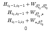
Equation 2.6 shows an example for a general 2-dimensional matrix H, see also figure 26 on page for the banding specialisation of the algorithm.

$$\left\{\vphantom{ \begin{array}{c} H_{i_{1}-1, i_{2}-1} + W_{\en... ...ensuremath{*}, \ensuremath{\mathcal{S}_{i_2}^{2}}}\\ 0 \end{array} }\right. \begin{array}{c} H_{i_{1}-1, i_{2}-1} + W_{\ensuremath{\mathcal{... ...2} + W_{\ensuremath{*}, \ensuremath{\mathcal{S}_{i_2}^{2}}}\\ 0 \end{array} \left.\vphantom{ \begin{array}{c} H_{i_{1}-1, i_{2}-1} + W_{\ens... ...nsuremath{*}, \ensuremath{\mathcal{S}_{i_2}^{2}}}\\ 0 \end{array} }\right\}$$ (6)

To calculate the value of H_{i1, i2}, it is only necessary to know the contents of the three predecessor cells (H_{i1-1, i2-1}, H_{i1, i2-1}, H_{i1-1, i2}).

While the multiple alignment problem is NP complete in the number of sequences, there is a well-known O(n^k) dynamic programming algorithm for computing alignments among k sequences of average length n (Smith and Waterman (1981)). The problem can be solved by simply extending the dynamic programming recurrence for the basic problem: computing the values of matrix H in some topological ordering requires a total relative time of

O($$\prod_{{i=1}}^{k}$$nⁱ) = O(n^k)

steps, where

n = max{nⁱ : i $$\in$$ [1, k]}

While the extension to multiple sequences is conceptually quite straightforward, the obvious algorithm to compute the exact solution takes an amount of time exponential in k. It is therefore generally impractical in real world problems for k > 3 (Myers (1991)) sequences and - even when restricting the computation space by some means - certainly so for k > 4 (Gotoh (1993)).