Read scanning

A common start for any assembly is to compare every read with every other read (and its reversed complement) using a fast and fault-tolerant algorithm to screen all reads and detect potential overlaps.

As Anderson and Brass (1998) denoted, ``the effectiveness of database search methods can also be illustrated by the distance the query sequences can be evolved before the search method no longer finds the homologous sequence in the database.''

In this section, the problem of finding similar subsequences including errors is formalised and existing algorithms are presented. Then two fast scanning algorithms - named DNA-SAND and ZEBRA - and their theoretical effectiveness are presented.

Formalising the problem

Let $\mathcal {A}$be the alphabet of an (unknown) true sequence T - which has passed through the electrophoresis and base-calling process - and of which we now have a representation $\mathcal {S}$^x in the alphabet $\mathcal {A}$^x.

In the notation of regular expressions: let a true sequence T of length n_t be denoted by T = t₁t₂...t_n (with $t_i \in \ensuremath{\mathcal{A}}\,$) and let the representation S be denoted by S = s₁s₂...s_m (with $s_i \in \ensuremath{\mathcal{A}^{x}}$). The three types of errors in $\mathcal {S}$^x of length m can be modeled as follows (assuming that a $\in$ $\mathcal {A}$^x):

• insertions into S with the operator ^* meaning zero or more occurrences of the preceeding character $a \in \ensuremath{\mathcal{A}^{x}}$

  S = a^*t₁a^*t₂...a^*t_na^* (7)

• deletions from S with the operator ? meaning zero or one occurrence of the preceeding character

  S = t₁?t₂?...t_n? (8)

• mismatches in S with (t_i| a^{a $\neq$ t_i}) meaning a choice between t_i and a character from $\mathcal {A}$^x which is unequal to t_i

  $$\neq \neq \neq$$ (9)

Typically, S does not contain only one type of errors but all three. The formally correct regular expression for this is

$$\neq \neq \neq$$ (10)

which can safely be shortened to

S = a^*t₁?a^*t₂?...a^*t_n?a^* (11)

during a string comparison process as

$$\neq$$ (12)

so that in the case of a mismatch, the preceeding a^* expression in front of t_i? would already catch any error.

In plain words: each base of the true genomic sequence T one wants to know may or may not be present in its representation S; additionally, it may or may not be surrounded by one or more artefact bases in S.

Finally, the orientation of S compared to T is unknown. S can be in the same direction as T, but it also can be in the reverse complemented direction. In this case, the bases in S must be reversed and complemented before a search can take place. Defining $\overline{t} \in \ensuremath{\mathcal{A}^{x}}$ as the complementary base of $t \in \ensuremath{\mathcal{A}^{x}}$, it is very well possible that

S = a^*t₁?a^*t₂?...a^*t_n?a^* (13)

but also that

$$\overline{{t}}_{n}^{} \overline{{t}}_{{n-1}}^{} \overline{{t}}_{1}^{}$$ (14)

The problem is now to design fast algorithms that can recognise patterns in sequences containing all errors described above.

Present algorithms

Several algorithms developed for string comparisons in computer science have been adapted to the needs of bioinformatics during the past decades, as searching large protein or nucleic acid databases has always been a critical application in biosciences¹⁷. There is one main differentiation to be made: depending on the type of search, searching in protein databases sometimes requires algorithms completely different from those for searching in nucleic acid sequences. Errors occurring in the nucleic acid sequence will cause - in the case of indels - a frame-shift on the protein level, subsequently changing all the following amino acids. At the nucleic acid level, an indel just inserts or deletes a base without changing the following bases. The following text focuses on the special problem of searching patterns in nucleic acid sequences.

In many cases, algorithms that work well for normal texts or in signal theory are not well suited for DNA sequences.

Multiple sequence alignments techniques that use the fast Fourier transformation (FFT) have been much less studied than other string and character based algorithms, although FFTs are a widely used method in signal data computation. A reason for this could be that Felsenstein et al. (1982) first published results of using simple variants of this method that cannot allow for insertions and deletions during matching and were not really satisfactory, but given the drastic increase in computation power in the last 20 years, Rajasekaran et al. (2002) and Katoh et al. (2002) were able to refine the approach and achieve good results.

The 'optimal mismatch' algorithm presented by Sunday (1990) relies on alphabet size and character frequencies in a text to achieve a searching speed which is in most cases well below O(n). But in most nucleic acid sequences gained from sequencing, the size of the alphabet is only 4 characters (plus one wildcard) and the frequencies of the bases are almost equally distributed. This noticeably reduces the effectiveness of the algorithm. Although it is relatively easy to implement single character wildcards like ``N'' (Gronek (1995b)) or the IUPAC code, it still cannot allow for indels.

Algorithms based on adapted Boyer-Moore string searching methods (Boyer and Moore (1977)) have also been implemented and used in the bioinformatics field (Prunella et al. (1993)), but these require a comparatively slow sequence preprocessing step. Giladi et al. (2002) presented an algorithm based on tree-structured index of k-tuple windows in vector space, with tree-structured vector quantisation which worked well only in balanced trees.

The dynamic programming algorithms for global alignments introduced by Needleman and Wunsch (1970) and later refined for local alignments by Smith and Waterman (1981) are the most suited methods for detecting - even partial - overlaps between sequences. They allow insertions, deletions and mismatches in both sequences and some algorithms, e.g. Guan and Uberbacher (1996), allow frameshift errors in protein sequences. Unfortunately, the run-time complexity of unbanded versions of those algorithms - this means, without prior knowledge or assumptions about the alignment of the sequences - is O(n*m), with n and m being the length of the two sequences. This makes the run-times unacceptable for most screening procedures when special hardware acceleration is not available.

Obviously, the problem of indels occurring in a sequence is one of the hardest ones to be solved. This is the reason why almost all programs available today for heuristic string searching are based on the word-based method introduced by Wilbur and Lipman (1983). The most known representatives for this search class are the FASTA family of programs (Pearson (1998)) and the BLAST family (Altschul et al. (1997)). They use (sometimes inverted) indices and the fact that matches between a search pattern and a sequence have at least one word of several error-free bases in common (Schuler (1998); Huang (1996)). Methods for allowing mismatches and indels (Grillo et al. (1996)) or basing on probabilistic interpretation of alignment scoring systems (Bucher and Hofmann (1996)) have also been devised, but are generally impracticable for more than one or two errors. The newer SSAHA algorithm by Ning et al. (2001) used a new way to combine position specific hashing algorithms using non-overlapping k-tuples and hit sorting algorithms. Recently, Kent (2002) developed the BLAT tool which performs ``stitching and filling in'' of multiple exact k-tuple matches to produce a fast aligner, but notes that the alignment strategy becomes less effective for sequence identity below 90%.

There is a major drawback of these methods: for finding matches in regions with high error rates, the specificity of the search has to be decreased to a point where true-positive matches are (by far) outnumbered by spurious, false-positive matches. This is often the case at the ends of shotgun-sequenced data.

DNA-Shift-AND algorithm

An interesting algorithm for searching patterns allowing errors is the Shift-AND algorithm presented in Wu and Manber (1992b) and Wu and Manber (1992a), based on previous work of Baeza-Yates and Gonnet (1992). The alphabet $\Sigma$ in which to search can be freely chosen, character frequencies of single letters in the text do not impede the speed of the algorithm. Searching for patterns in a text is abstracted to the problem of iterating bit arrays according to a predetermined schedule (Gronek (1995a)) stored in transition tables. These arrays represent different states of search results of a pattern against a text and can thus be held in machine registers if the length of the pattern does not exceed 32 or 64 characters, depending on the processor type.

The Shift-AND algorithm searches a pattern of configurable length in a sequence allowing for a configurable number of errors. Since most BLAST search actions in nucleotide sequences are performed with a word length well below 32 characters, the length of patterns has been limited to 32 bases. This allows to write the algorithms in a way that fits to the architecture of virtually all presently available machines. The algorithm has been implemented in a straight-forward way based on the publications of Wu and Manber (1992b) and Gronek (1995a).

Due to limitations of the pattern length discussed above, the complexity of the DNA-Shift-AND (DNASAND) algorithm as it has been realised is O(cn); where c is the number of errors allowed in a pattern and n is the length of the text to be searched. The algorithm is nonetheless able to recognise regular expressions as defined in equations 4.7 and 4.8, as long as the number of correct bases and the number of errors does not exceed the length of a pattern to be searched. For example, searching for a DNA pattern of length 20 and allowing 3 errors will find any occurrence of the pattern in a sequence with 17 correct bases and 3 errors, 18 bases and 2 errors, 19 bases and 1 error or the complete pattern without errors. Each error might be either an insertion, a deletion or a mismatch at any location. This metric to measure the similarity between two strings is called the Levenshtein distance when each insertion, deletion or mismatch is defined to count as one error.

Implementation of the DNASAND sequence filter

The function of a DNA sequence overlap filter is to find as many potential overlaps between sequences as possible. A key point in this requirement is the ability to find - besides long overlaps with low error rates expected to be recognised by any algorithm - even weak overlaps between any two sequences. Weak overlaps are characterised either by only a small number of bases from each sequence overlapping each other or by overlapping bases having a high error rate; or both. Of all the string comparing and string alignment algorithms known up to now, only the Smith-Waterman dynamic programming algorithm has the possibility to find even weak overlaps. Unfortunately it has too high processor requirements to be used as a fast filter. The DNASAND algorithm is a good substitute for this task.

A reasonable assumption for determining overlaps would be that two sequences S₁ and S₂ might overlap if they both have a succession of k bases in common (a common subsequence). As the probability of the sequences having errors is high enough, it is wise to extend the assumption: S₁ and S₂ might overlap if they have a common subsequence k bases long with at most l errors in it. The problem is now to find the common subsequence.

As the problem is to find even weak overlaps, a first approach would be to take the first k bases of S₁ as pattern P_1s and search for it in S₂ (allowing l errors). The localisation of the two sequences relative to each other is unknown, it is therefore necessary to do the same the other way round: take the first k bases from S₂ as pattern P_2s and - allowing l errors - and search for it in S₁. Doing this, every overlap combination of two sequences having the same orientation (both forward or in reversed complement direction) and at least k bases in common with at most l errors will be found.

The next difficulty is the fact that the orientation of the sequences to each other is unknown: they both can have the same direction - for the sake of simplicity, it is indeed of no consequence to the filter whether the sequences are both in forward or both in reversed complement direction, as long as it is the same orientation - or they can have opposite directions where one of the sequences overlaps with the reverse complement of the other sequence¹⁸. To find overlapping sequences that do not have the same direction, the pattern P_s taken from a sequence S_i must be searched in S_j and the reversed complement pattern $\overline{{P}}_{s}^{}$ from S_i must be searched in S_j.

Figure 15: Mode of operation for DNASAND. When searching for overlaps for two sequences, patterns from the start, mid and end of each sequence are taken and slided across the other sequence with the Shift-AND algorithm. The same is done for the reverse of the sequences (not shown).

Doing this, there is still one further possibility for two sequences to overlap that would not be found using this method: when two sequences having opposite directions overlap at the end.The solution to this problem is to take not only the start of a sequence to search as pattern P_s or reversed complemented pattern $\overline{{P}}_{s}^{}$ in any other sequence, but also to take the end of a sequence as pattern P_e or as a reversed complemented pattern $\overline{{P}}_{e}^{}$ and search for it in each other sequence.

Summarising the above considerations: to determine if a sequence S_i might overlap with any other sequence S_j, two patterns - P_is at the start and P_ie at the end - and their reversed complements - $\overline{{P}}_{{is}}^{}$ and $\overline{{P}}_{{ie}}^{}$ - are taken from S_i. These patterns are compared with the modified Shift-AND algorithm to the whole sequence S_j and will show if the patterns match anywhere within S_j. If this is the case, the filter can assume that there is a potential overlap between S_i and S_j (or between $\overline{{S}}_{i}^{}$ and S_j).

However, there is still one problem to consider: the filter relies on the potentially poorest data - present at the end of sequences - to find even the weakest overlaps. It is always possible that the ends of the sequences contain too many errors to act as reasonable patterns, which, in turn, can cause the filter not to recognise potential overlaps. Some prerequisites have to be met for a situation like this to happen: the ends of the sequences are polluted with foreign DNA like non-removed vector sequence, or they contain an unusually high level of errors which has not been recognised by programs performing quality-clipping.

It is, consequently, wise to take preventive measures for cases like these. A third pattern and its reversed complement to be searched for are hence introduced in each sequence. These patterns P_im and $\overline{{P}}_{{im}}^{}$ are taken from the mid of each sequence S_i; thus in a region where the error rate is presumably very low. This third pattern acts as safety net: it will not find weak overlaps, but it will recover potential overlaps that have slipped through the patterns from the ends of the sequences because of a too high error rate. Figure 15 gives an overview on the resulting mode of operation for DNASAND.

The ZEBRA algorithm

Grillo et al. (1996) presented an algorithm to find and remove redundancies in genomic databases. This algorithm is based on an 'approximate string matching' procedure, which is able to determine the overall degree of similarity between each pair of sequences contained in a nucleotide sequence database. The basic idea of their computational model is the generation of a set of highly descriptive indices for each sequence position by hashing each position in a nucleotide string and using wildcards.

Although the original method is too slow to be directly applicable to the problem of finding similarities in shotgun data, a way has been found for this thesis to extend and combine it with algorithms coming from the field of theoretical signal analysis. The ZEBRA¹⁹ algorithm that was developed is based on the insight that within normal shotgun data, the number of reads not matching with each other increases with the square of the number of reads present, while the number of reads matching increases only linearly. It is therefore important not to recognise matching reads quickly, but to skip non-matching reads as fast as possible.

The strategy used is not a divide and conquer but rather a transcribe, divide, reorganise, concentrate and conquer strategy. As bonus, ZEBRA calculates the offset of the overlap on the fly.

Implementation of a ZEBRA sequence filter

As shown in figure 16, the alphabet of a nucleotide sequence can be translated into hash values of any desired length by segmenting it into tuples. The cardinality of the nucleotide alphabet is 4 (2 bit). Assume that one can code an A to 00, C to 01, G to 10 and T to 11. This enables to hash 8 nucleotides (nucleotide 8-tuple: an octet) into a 16 bit integer value (the reason for using 16 bits - apart from the fact that this is standard word size for computer systems - will be explained later on).

Figure 16: Transforming a nucleotide 8-tuple (octet) into a 16 bit hash.

Doing this for every position of a nucleotide sequence of size n will result in n - 7 hashes, but - similarly to the strategy used in the DNA-SAND algorithm - an N in the nucleotide sequence is treated as correctly recognised but otherwise unspecified base. Therefore, not one hash is computed for a nucleotide octet containing one N, but four (see figure 17): by sequentially substituting the 'N' for one of the bases A, C, G and T. Although more than one N within an octet could be computed using the same logic, this would increase dramatically the number²⁰ of hashes to be computed. Fortunately, more than one N within a short number of nucleotides can be seen as hint that the base caller had severe problems to find the right bases because of bad signal quality. As a consequence, nucleotide octets containing more than one N are not computed.

Figure 17: Transforming a nucleotide octet containing one undefined base into four 16 bit hashes.

Figure 18 demonstrates how hashes are stored in a table (the combined hash-position table) together with the index position at which they occur. Once the sequence has been transformed into the table, it is sorted using the hashes as key.

Figure 18: Computation of the combined hash-position table by successively computing nucleotide octet hashes for each position of a sequences and storing the hash values together with the position at which they occurred in a table. Then sort the table using the hashes as key.

Figure 19 shows how the resulting sorted table is split up into two subtables: a hash index table (which will subsequently be called imprint) and a hash position table. The imprint contains exactly k = 2ⁿ elements with n being the number of bits in a hash value. In the case of the ZEBRA algorithm, n = 16 so this results to k = 65536 elements per table. Each element in the imprint is either a NULL pointer - if the corresponding hash has not been computed - or a pointer to the first hash position element in the hash position table. The hash position table is composed by the hash positions sorted in ascending order with a special element (-1) as delimiter to mark the end of the corresponding hash.

Figure 19: Splitting a combined hash-position table into a hash index table (an imprint) and a hash position table.

Comparing two sequences is now reduced to the task of comparing two imprints element by element and logging the distance at which equal hash positions appear in two sequences. A NULL pointer in one of any two imprint elements shows that the corresponding nucleotide octet does not appear in the sequence belonging to the imprint, whereas a valid non-NULL pointer into a hash position table within both elements of an imprint shows that at least the octet belonging to this hash appears in both nucleotide sequences.

As the length of todays shotgun sequences varies between 300 and 1500 bases, imprints of size k = 2¹⁶ will have only between ${\frac{{1}}{{64}}}$ and ${\frac{{1}}{{40}}}$ of their elements filled with non-NULL pointers. As result, sequences being completely dissimilar will generate only a few hits when comparing their imprints. Assuming a random distribution of hashes, the number of equal hashes in two imprints is expected to be

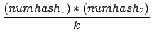$${\frac{{(numhash_1)*(numhash_2)}}{{k}}}$$        with k = 65536 in this case

For example, one can expect between 1.7 (300 bases) and 34.3 (1500 bases) occurrences of the same octet in non-related sequences.²¹

In case a hash is present in both imprints, the relative distance between the two octets can be calculated by stepping through the corresponding positions in the hash position table and subtracting the position of the octet in the first sequence from the position of the same octet in the second sequence. This must be done for all appearances of this octet in both sequences. The relative distance at which two equal octets occur in a sequence is logged in a histogram (see figure 20).

Figure 20: Computational scheme for the octet relative distance histogram of two sequences. Dissimilar sequences with dissimilar octets will show single occurrences scattered across the histogram. Similarities between two sequences will show up as peaks of variable height and width. The higher the peak, the more similar octets have the same relative distance. The wider the peak, the more insertion and deletion errors are in one or both of the two sequences.

Therefore, the algorithm does not explicitly track occurrences of longer subsequences, but looks at the similarity as whole between two sequences. This keeps data structures and code loops simple enough to let compilers optimise at their best.

Note that the problem of comparing two sequences has been reduced to a loop operation that fetches successive data from memory and compares it. Any of todays processors uses speculative data prefetch (sometimes called data burst), i.e, if data is fetched from address n in memory, the processor will speculatively prefetch a certain number of data beginning at n + 1 in its 'spare time' as many algorithms work on consecutive data in memory and the probability of needing this data within a short period of time is fairly high. The ZEBRA algorithm is designed in exactly this way to support that feature and this effectively leads to a speed increase of the algorithm: in dissimilar sequences, the algorithm spends most of the time by comparing the two imprints and only exceptionally looks up data in the hash position table, computes octet distances and stores them in the distance histogram.

The histogram itself shows the result of the comparison of two sequences in a very straightforward way. The three distinct types of histogram are:

1. Similar octets occurring in both sequences but at different relative distances from each other. The occurrences are scattered across the histogram, no distinct peak can be detected. Thus, the sequences do not resemble each other and are not possible overlapping candidates.
2. A single peak. The higher the peak, the more nucleotide octets pairs have the same relative distance and the wider the peak the more insertion and deletion errors occur in one or both sequences.
3. A certain number of peaks, sometimes not clearly separated. This is typical for identical short term repeats between 1 and a few dozen nucleotides occurring in both sequences. The repeated occurrence of equal octets at different places in the sequences leads to a smearing effect.

Once a peak in the histogram exceeds a configurable height, the two sequences can be seen as potentially overlapping. The higher the peak, the more octets in both sequences have the same relative distance from each other. The wider the peak, the more insertion and deletion errors are in one or both of the two sequences. The offset of the peak and its height give - together with the length of both sequences - a valuable first guess of the overlap strength.

Improving the ZEBRA sequence filter: speeding up comparison

An important insight is the fact that comparing two imprints is implemented by iteratively making boolean decisions regarding the state of two array elements. In fact, an imprint element containing a NULL pointer can be expressed as 0 (or false), while an imprint element containing a valid pointer into the hash position table can be expressed as 1 (or true).

$$\mbox{compressed\_imprint}[k]=\left\{ \begin{array}{l}\mbox... ... imprint[$k$] != NULL}\\ \mbox{false else}\end{array} \right.$$

This leads immediately to the approach of compressing the imprints into bit vectors as performing AND operations on multiple bits (8, 16, 32 or even 64 bits). Logical operations like AND are one of the most common and thus fastest operation realised within hardware. Figure 21 shows the compressing process exemplarily.²²

Instead of comparing 2 times 128kB, the same operation can be done by performing an AND operation on 2 times 8kB. This reduces greatly the number of loop iterations and the amount of data transported on the system bus between RAM and processor.

Figure 21: Compressing the imprint by transforming pointers into boolean arrays.

The number of potential overlaps grows linearly to the number n of sequences an assembly project contains, while the number of non-overlapping reads approximates to n². It is therefore preferable to speed up the comparison of two dissimilar sequences than the comparison of two similar sequences.

In fact, ZEBRA implicitly allows to take advantage of the data structures created to support this goal. As already proven, major parts of any sequence imprint are filled with NULL pointers (respectively 'false' in a compressed imprint) so that comparing dissimilar sequences will generate only sporadically false positive octet hits. The idea is now to compress the compressed imprint further to reduce the number of loop iterations and data transports between RAM and processor even more.

Consecutive bits in a compressed imprint can be bundled by the OR operation: bundling n consecutive bits leads to a compressed_imprint_n. Comparing two sequences is then done by comparing two compressed_imprints_n. If both have a bit set at the same position, then the corresponding imprint elements have to be examined more closely. This is - of course - affected with an overhead: data speculatively prefetched by the processor must be discarded and data stored in other tables must be fetched. If n is chosen too low, the full potential of compression and loop iteration decrease is not used. On the other hand, if n is chosen too high, the imprints will be compressed too much: this leads to an exaggerated number of false positive hits in the comparison of two compressed_imprint_n.

During experiments with projects between 500 and 5,000 reads, having an average usable sequence length between 300 and 1,000 bases, nesting a compressed_imprint₁ loop within a compressed_imprint₈ loop gave the best overall time performance.

Improving the ZEBRA sequence filter: dealing with errors

Up to this point, the ZEBRA algorithm still cannot handle insertion or deletion errors very well. Still, it is known that the sequences that are to be compared are potentially error prone, especially toward the ends. This may include insertion and deletion errors.

This can be addressed quite easily by using a technique made popular by Grillo et al. (1996). The technique presented in that paper consists of computing not one hash per sequence position, but expecting the nucleotide tuple to contain errors and taking this into account by computing multiple hashes, each hash representing the possibility of a certain number of errors being contained in the tuple.

As already seen in section 2.2, sequences gained in laboratory tend to have less than 1% errors within the good middle part, but up to 15% toward the ends before the reads become completely unusable.

Following the conclusions of Grillo et al. (1996), computing n₁-tuples - this means, tuples containing n nucleotides but allowing 1 error - is a good compromise between sensitivity, specificity, computational overhead and execution speed. Porting this to the ZEBRA algorithm, this results into using 9-tuples allowing 1 error (see figure 22).

Figure 22: Transforming a nucleotide 9-tuple into 9 hashes describing the tuple allowing for 1 error.

Doing this for any position in each sequence allows the ZEBRA algorithm to deal with insertion/deletion errors, but also increases the number of hashes present in an imprint by approximately a factor of 8 to 9.